Stiffness Matrices
The ABD stiffness matrix relates the applied loads to the laminate mid-plane strains and curvatures. It is assembled from individual ply contributions using CLT.
Ply Reduced Stiffness (Q & Q̄)
The reduced stiffness matrix [Q] defines the elastic properties of a single orthotropic ply in its principal material axes (1-2 coordinate system). The terms are derived from the basic engineering constants:
Q₁₁Q₁₂0Q₁₂Q₂₂000Q₆₆ | where | Q₁₁ = E₁ / (1 − ν₁₂ ν₂₁)Q₂₂ = E₂ / (1 − ν₁₂ ν₂₁)Q₁₂ = ν₁₂ E₂ / (1 − ν₁₂ ν₂₁)Q₆₆ = G₁₂where ν₂₁ = ν₁₂ · E₂ / E₁ |
When a ply is rotated by an angle θ relative to the laminate x-axis, its stiffness is transformed into the global x-y coordinate system. This yields the transformed reduced stiffness matrix [Q̄]:
ABD Stiffness Matrix
The constitutive relationship of CLT is expressed as:
NxNyNxyMxMyMxyVxVy | = | A₁₁A₁₂A₁₆A₁₂A₂₂A₂₆A₁₆A₂₆A₆₆B₁₁B₁₂B₁₆B₁₂B₂₂B₂₆B₁₆B₂₆B₆₆000000 B₁₁B₁₂B₁₆B₁₂B₂₂B₂₆B₁₆B₂₆B₆₆D₁₁D₁₂D₁₆D₁₂D₂₂D₂₆D₁₆D₂₆D₆₆000000 000000000000H₄₄H₄₅H₄₅H₅₅ | ε⁰xε⁰yγ⁰xyκxκyκxyγxzγyz |
- [A] — Extensional Stiffness (lb/in) — Relates in-plane forces to mid-plane strains. Symmetric 3×3 matrix.
- [B] — Coupling Stiffness (lb) — Couples in-plane forces to curvatures and moments to mid-plane strains. Zero for symmetric laminates.
- [D] — Bending Stiffness (lb·in) — Relates bending moments to curvatures. Symmetric 3×3 matrix.
- [H] — Transverse Shear Stiffness (lb/in) — Relates transverse shear forces (V) to transverse shear strains (γ). Symmetric 2×2 matrix.
Each sub-matrix is computed by summing the contributions of all N plies, weighted by their transformed reduced stiffness [Q̄] and their vertical position through the thickness (from zk-1 to zk):
Compliance Matrix (abd)
The compliance matrix is the inverse of the full 6×6 ABD matrix. It is partitioned into four 3×3 sub-matrices:
- [a] — Extensional compliance (in/lb)
- [b] — Coupling compliance (1/lb)
- [c] — Coupling compliance = [b]ᵀ (1/lb)
- [d] — Bending compliance (1/(lb·in))
The mid-plane strains and curvatures are obtained by multiplying the compliance matrix by the load vector: { ε⁰, κ } = [abd] · { N, M }.
Effective Engineering Constants
Effective engineering constants are derived from the laminate compliance matrix [a] (the upper-left 3×3 sub-matrix of [ABD]⁻¹) and the total laminate thickness h. This approach is valid for all laminates, including non-symmetric and unbalanced layups.
| Constant | Formula | Description |
|---|---|---|
| Ex | 1 / (h · a₁₁) | Effective modulus in x-direction |
| Ey | 1 / (h · a₂₂) | Effective modulus in y-direction |
| Gxy | 1 / (h · a₆₆) | Effective in-plane shear modulus |
| νxy | −a₁₂ / a₁₁ | Effective Poisson's ratio |
| νyx | −a₁₂ / a₂₂ | Reciprocal Poisson's ratio |